Deployment vs. Utilization: Let’s Compare the Two Numbers That Drive Equipment Profitability

Key takeaways: 

• Deployment is the foundation of profitability. Equipment can't be utilized if it isn't in the right place at the right time.
• Deployment and utilization work together. Fleets recover ownership costs when machines are both deployed to jobsites and actively working.
• Measuring both metrics reveals performance gaps. Low deployment and low utilization point to different problems that require different solutions.

We have always said that utilization holds the key to success when it comes to recovering fixed costs and balancing the equipment account. Perhaps we have been wrong. Perhaps deployment holds the key. The logic is simple: You cannot use a machine unless you have the right machine in the right place at the right time. The efficient planning, communication, and dispatch operations needed are critical for success and must be managed accordingly. Confusing deployment and utilization and blending them into one metric can lead to misunderstandings that make it impossible to measure and improve performance. So, let’s start with a couple of definitions.

Deployment vs. utilization: What’s the difference?

Deployment: The time a machine spends in the right place at the right time. It depends on planning and communication between Operations and Equipment, having the right equipment available, and the logistics needed to dispatch equipment as and when required.

Utilization: The time the machine spends working and producing completed construction, safely, on time, on budget, and to the required quality. It depends on the ability of the project team to use the resources they have and get the job done.

Deployment is usually measured in weeks per year. The benchmark values seek to answer the question, “How many weeks per year do you expect this machine will be on site and contributing to activity on the site?” The data required to measure deployment relies on a knowledge of where each machine is each day.

Utilization is usually measured in hours worked per week. The benchmark values seek to answer the question, “How many hours per week do you expect that this machine will be used to produce completed construction while it is on site?” The data required to measure utilization comes from your knowledge of the status of a particular machine — what is it doing, is it being used?

The math behind equipment cost recovery

Expected deployment and expected utilization give you an extremely critical number when you multiply them together. If you expect the machine to be on site for 45 weeks per year and you expect it to work for 40 hours per week while on site, then you are saying that you expect the machine to work for 1,800 hours per year (45 x 40). This is, or should be, the number you use to convert fixed annual owning costs into an hourly rate in your rate calculation.

So, we can say that if you achieve the expected deployment and expected utilization, then you will recover the fixed annual owning costs, and the owning cost side of your equipment account should balance. Let’s use a simple example to see how it all works.

A real-world deployment example

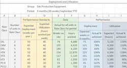
The table headings above tell us that we are measuring Deployment and Utilization for a Group of Site Production Equipment for a nine-month (or 39-week) period ending in September. Column A lists the Rate Classes that fall in the group. We see there are three excavator classes (Large, Medium, and Small), three haul truck classes (40, 30, and 20 ton) and two paver classes (8 and 12 foot). Column B lists the number of units that we own in each Rate Class. Columns C and D give the Performance Standards for deployment and utilization that were defined when setting up each Rate Class. 

You can see that the expectation is for all units to be deployed on site for 45 weeks per year except for the large excavators (EXL), 40-ton haul trucks (HT4), and pavers (PV8 and PV12). The expectation is that the excavators and loaders will work for 50 weeks per year while the pavers will only work 30 weeks per year due to winter constraints. The utilization benchmark (Column D) is 40 hours per week for all units except, again, for the pavers where constraints on shift planning limit utilization to 30 hours of working time per week.

The expectations in columns C and D show that we are expecting the large machines to work a total of 2,000 hours per year (50 weeks per year times 40 hours per week) while expecting the pavers to work only 900 hours per year (30 weeks per year times 30 hours per week). The rate calculations for these Rate Classes will be based on these values and the fixed annual owning costs of ownership will only be recovered if Deployment times Utilization equals the expected hours per year.

Columns E and F give the data required in the calculation. Column E is the actual number of weeks on site recorded for all the units in each Rate Class during the period covered by the report. Column F is the actual number of hours worked by all the units in each Rate Class during the period covered by the report. The values are easily obtained from GPS telematics systems and will, of course, have been reconciled with data collected by site superintendents as they complete their job cost reports. Columns G and H show the deployment calculation. The expected number of weeks for each Rate Class is:  Column B times Column C times 9 for the 9 months to September divided by 12 for the number of months in the year. For EXL, this comes to 2 units times 50 weeks in the year (equals 100) times 9 over 12 to reflect the fact that the report is for 9 months, YTD. (2 x 50 x 9 / 12 = 75).

The actual deployment percent achieved is simply Column E over Column G. The EXL, HT4 and HT3 rate classes have all been on the same high tempo job for the whole 39-week period and so they have similar high deployment percentages. The paving season got off to an early start. The two PV8s have been on site for 55 weeks out of the 45 expected weeks to give a deployment of 122 percent. The PV12 has also been deployed for more weeks than expected and its deployment is also very high.

Columns I and J show the utilization calculation. Clearly, a machine cannot be utilized if it is not on site. Therefore, the expected utilization in hours in Column I is simply Column D times Column E. The actual utilization percent achieved is Column F divided by Column I. The high tempo job on which the EXL, HT4, and HT3 rate groups have been working has clearly exceeded utilization expectations. The early start to the paving season, while good for the deployment, has resulted in poor utilization — probably due to late starts on cold mornings.

The interesting insights come when you look at the chart below.

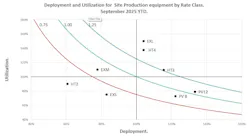
What the chart reveals

The % Deployment and % Utilization for each Rate Class is plotted on the chart with the horizontal axis showing percent deployment and the vertical axis showing percent utilization. 

The green downward-sloping line shows when the % deployment times % utilization equals 1. In other words, when expectations are met and the fixed annual owning costs are fully recovered.  The blue line shows when the product of the two percentages comes to 1.25 (in other words, you are making a bit of money on owning costs). The red line shows when the product of the two percentages comes to 0.75 (in other words, you are losing a lot of money on owning costs). The three rate classes on the high tempo job (EXL, HT4, and HT3) are doing great. Both utilization and deployment expectations are being met and the fixed annual owning costs are more than recovered. You may want to start a discussion about lowering the rate or returning some of the over-recovered owning costs to the job.

Finding problem machines

The pavers are doing well despite low utilizations. The early deployments have kept them close to the green line despite low utilizations. The mid-size excavators (EXM) are hanging on. The effect of low deployment is being mitigated by relatively high utilizations. It seems that there are problems with the small excavators (EXS) and small haul trucks (HT2). Deployment for the small excavators is not bad but utilization is low — is there a job that has one on site but is not using it? With regard to the small haul trucks (HT2) — deployment is very low — is there really work for four small haul trucks? Are there any that have been standing in the yard? What about the two that are being rebuilt at the dealership?

Success requires both metrics

First, you have to have the right number of machines in the right place at the right time. You measure that with deployment. Second, you have to use the machines that you have got in the right place at the right time. You measure that with utilization. The methodology presented here is simple and straightforward. You know how many weeks per year you want the machines on the jobsite and you know how many hours per week we want them to work. You used those two numbers when you did the rate calculation. You have the required location and status data so you know where the machines are and we know how many hours they work. Do the calculations, plot the graphs, and find out what you need to do to balance the owning cost side of the equipment account.