Focus on Available Machine Hours
What do you buy when you buy a wheel loader? Do you buy one unit? Or do you buy a certain number of productive wheel loader hours that you put into inventory and keep there as an asset until it is used up in the production of work? The accountants certainly see the new wheel loader as an asset that will be depreciated over time. Fleet operations should also see it as such and think less about the number of units it owns and more about the productive hours it has in inventory in each rate class in the fleet.
Mike Vorster is the David H. Burrows Professor Emeritus of Construction Engineering at Virginia Tech and is the author of “Construction Equipment Economics,” a handbook on the management of construction equipment fleets. Mike is lead presenter at the annual Construction Equipment Management Program (CEMP) and serves as a consultant in the area of fleet management and organizational development.
The number of units we own in a given rate class certainly is important. We need a given number of wheel loaders to service the work sites we have; we need a given number of trucks to meet the daily haulage plan. On the other hand, hours in inventory is the critical metric when it comes to long-term fleet age management and capital expenditure planning.
Let’s see how it works and what we need to do to implement the concept.
1) Decide on the number of hours you put into inventory when you acquire a new machine. There are three ways you can do it.
Most defensible is to do a formal “sweet spot” analysis based on your knowledge of the way hourly owning costs decline and hourly operating costs increase over the life of the machine. This will ensure that lifecycle cost is minimized and that you plan to keep the machine for its formal economic life.
Another method is to put into inventory the same number of productive hours as you used when calculating the internal rental rate and thereby ensure that inventory hours line up with the lifecycle used in the hourly owning cost calculation.
The last method is to use best judgment and ask, “How many hours or miles do I think I can reasonably expect to get out of this unit before it becomes too expensive or unreliable to keep in my fleet?”
Of course, the formal, defensible methodology is best. Of course, the practical, experienced-based estimate is most often used. The bottom line is that it probably does not make a lot of difference. Analysis and experience should give us essentially the same answer. Know what you are doing, be prepared to justify your decision, and do not let the need to establish a target life stop you from implementing the concept.
2) Decide if and how you are going to add to your inventory when you do major component replacements or rebuilds. You will most certainly be adding to the quality and capability of units, the rebuilds will—most likely—be capitalized, and there will be an expectation of additional life. So adding to inventory is reasonable. Make good estimates and have the courage to explicitly increase life expectation when you rebuild a machine and explicitly add to inventory. Clearly, if you do not have a rebuild policy for units such as pickups, this is not an issue.
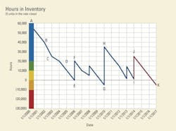
3) Record hours worked to date, do the numbers, and present the results on a good hard-hitting graphic. Consider the above diagram, which serves as a small, stylized example, to see how the format works and understand what it tells us.
- There are five units in this rate class, brought into service on 1/1/2000 with the assumption that each had 12,000 hours of productive life. The hours in inventory line thus starts at the top left at 60,000 hours (5 units at 12,000 hours each) at point A.
- The colored bar at the left sets arbitrary control limits that help trigger action. The green zone indicates when the units are, on the average, near their target life. It starts at 20,000 when each unit will, on the average, have 4,000 hours of life remaining. This means they will be 8,000 hours old (4,000 hours remaining means that 8,000 hours have been used up out of the original 12,000 hours). The yellow zone indicates the units have 2,000 hours left and are, on the average, 10,000 hours old. The orange zone starts when all the hours in inventory have been used up and the average age of the units is 12,000 hours. The red zone shows when things become critical and the original economic life expectation has been exceeded.
- The hours in inventory line starts at 60,000 hours (Point A, 5 units at 12,000 hours each) and works downward as the machines work and use up inventory. Point B, the end of the second year, shows that 20,000 hours have been used up and that 40,000 hours remain. This gives a utilization for the rate class of 10,000 hours per year (20,000 hours in 2 years) or 2,000 hours per year, on average, per unit. We hope that this is a good and acceptable utilization of the capital investment made two years previously.
- The downward slope of the line equates to the “burn rate” or hours consumed in the year. We see that utilization was very good in 2002 (B to C) when 15,000 hours (40,000 minus 25,000) were “burned up” between the 5 units at an average utilization of 3,000 hours per unit per year. On the other hand, we see that utilization was not as good in 2003 (C to D) when only 5,000 hours were burned up at a rate of 1,000 hours per unit per year.
- Nothing can be done about the fact that equipment assets are (indeed, should be) used up in the production of work. The hours in inventory line must thus slope downward over time. This has happened, and the rate class went into the yellow zone at the start of 2005.
- The class would have gone into the orange zone at the start of 2006, but 20,000 hours of inventory were added by selling a 10,000-hour unit and replacing it for a net gain of 10,000 hours, plus doing a major component rebuild on two units for a gain of 5,000 hours in each unit. The result is shown in the step from E to F.
- Utilizations varied for the next two years when the other two original units were rebuilt to add 10,000 hours to inventory at the end of 2008.
- Utilization was good for 2008 and 2009, and the group was well into the orange zone at the end of 2009 ( point G). Inventory was at minus 5,000 hours, and something had to be done to stay out of the red zone and avoid serious reliability and operating cost problems.
- Inventory was added and productive capability was restored at the beginning of 2010 by selling and replacing three units and rebuilding one to produce the 41,000-hour vertical step (from -5,000 to +36,000) given by the line from G to H. Average age was restored and the renewed fleet was good to go.
- Things continued to the present with one machine being replaced to add 12,000 hours of inventory at the start of 2013.
- The situation at the start of 2014 shows that the rate class is again about to go out of the orange zone and that, again, action is required. Workload projections for the years ahead are very good as given by the line J to K. Clearly, the right thing to do is to add to inventory by replacing some units. If two are replaced as shown by the line I to J, then the class will be back in the green zone—but only just. Trouble lies not far ahead. Inventory will be negative again before the beginning of 2017.
The hours-in-inventory graph gives us a lot of information. Most importantly, it requires us to think about the future and answers questions such as What have we got? What is our burn rate? and Where will we be in the future? Above all, it shows the relentless, ongoing need to replace our assets, maintain the capacity in our fleet, and stay out of the red zone.
Yes, you may be able to live off your new fleet and have the line trend downward for a while. But once you have done that, you cannot defer replacement for long. Above all, you cannot deny the fundamental rule that you must put into your fleet at least as much as you take out.